OFDM Wireless System with GNU Radio
Table of contents
0 Introduction
In this post I will deep dive into how to construct an Orthogonal Frequency Division Multiplexing (OFDM) wireless system using GNU Radio and two HackRF Software Defined Radios (SDR). We will eventually try to transfer an image over-the-air using QPSK modulation, and then demodulate the signal to recover the image.
We will first build the system and simulate it using GNU Radio. Then, we will modify it to work with actual SDR hardware.
1 Simulation
1.1 Transmitter
Before attempting to transmit the image, let us first look at a simpler payload in the form of a text file. I have generated a text file with 512 ASCII characters, as shown below. (Fun fact: I generated this text using Gemini.) I added a bunch of zeros at the beginning and the end of the text file, so that we can visualize it better when it is converted to a stream of numbers.
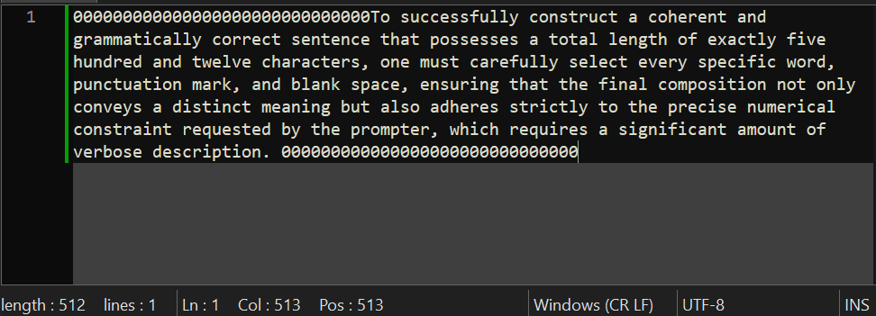
This text file is read by a “File Source” block in GNURadio, which outputs a stream of bytes (integers between 0 and 255). Note that each ASCII is one byte, or 8 bits.
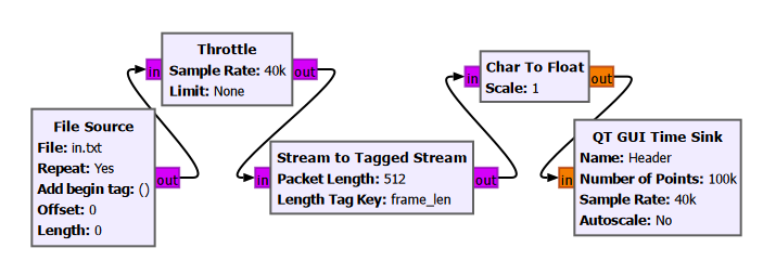
The output of the file source is fed into a “Stream to Tagged Stream” block, which adds a tag stream parallel to the main data stream (our text). In our example, we will add a tag to each packet of our input stream, with the tag value being the length of the packet. Our packet length is set to 256, meaning the whole text file can be described using two packets.
Let us visualize the tagged input stream using a “Time Sink”.
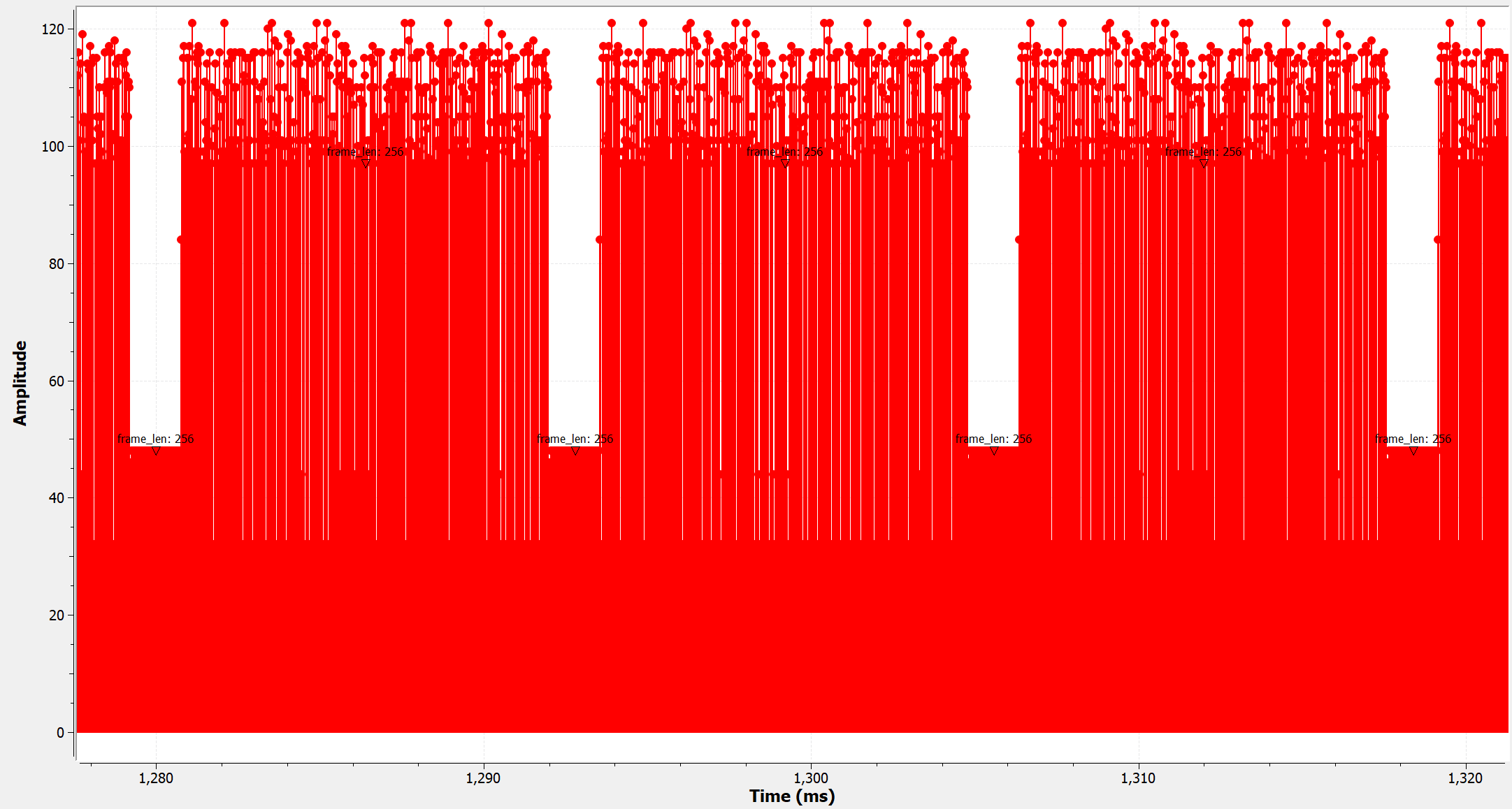
Since I set the File Source to repeat indefinitely, we can clearly see a periodic sequence of data samples with period 512. Each period begins and ends with the value 48, which is the ASCII value of the character “0”. We can also see the tags that are added to the data stream, which occurs once every 256 samples, i.e. there is a tag for each packet.
Next, we add a cyclic redundancy check (CRC) code to all of our packets, using the “Stream CRC32” block. This block takes each of our packets, computes a 32-bit CRC code, and adds it to the end of the packet. When the data + CRC code is received later, the receiver will try to perform calculations to decide if the received data has been corrupted. There are several ways this decision can be made at the receiver. I will not go through that here.
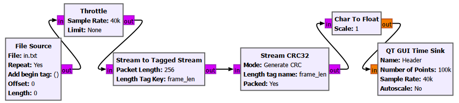
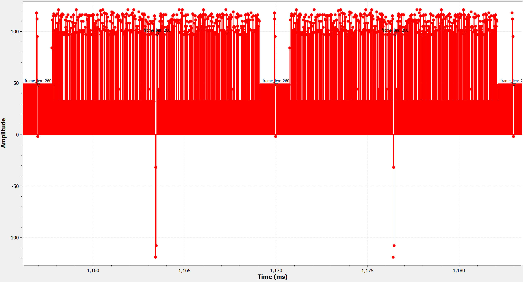
The output of the CRC block is shown below. Notice that each packet is 260-byte long, with the last 4 bytes being the CRC code.
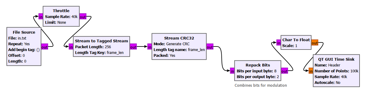
With the CRC code added, we can now convert our stream of bytes into a stream of QAM symbols. For this example, we will use QPSK modulation, which maps each pair of bits to one of four possible points on the IQ (complex) plane. Before mapping to the complex plane, we first convert each byte (8 bits) into four consecutive bit pairs (which will later be mapped to 4 consecutive symbols). We do this using the “Repack Bits” block.
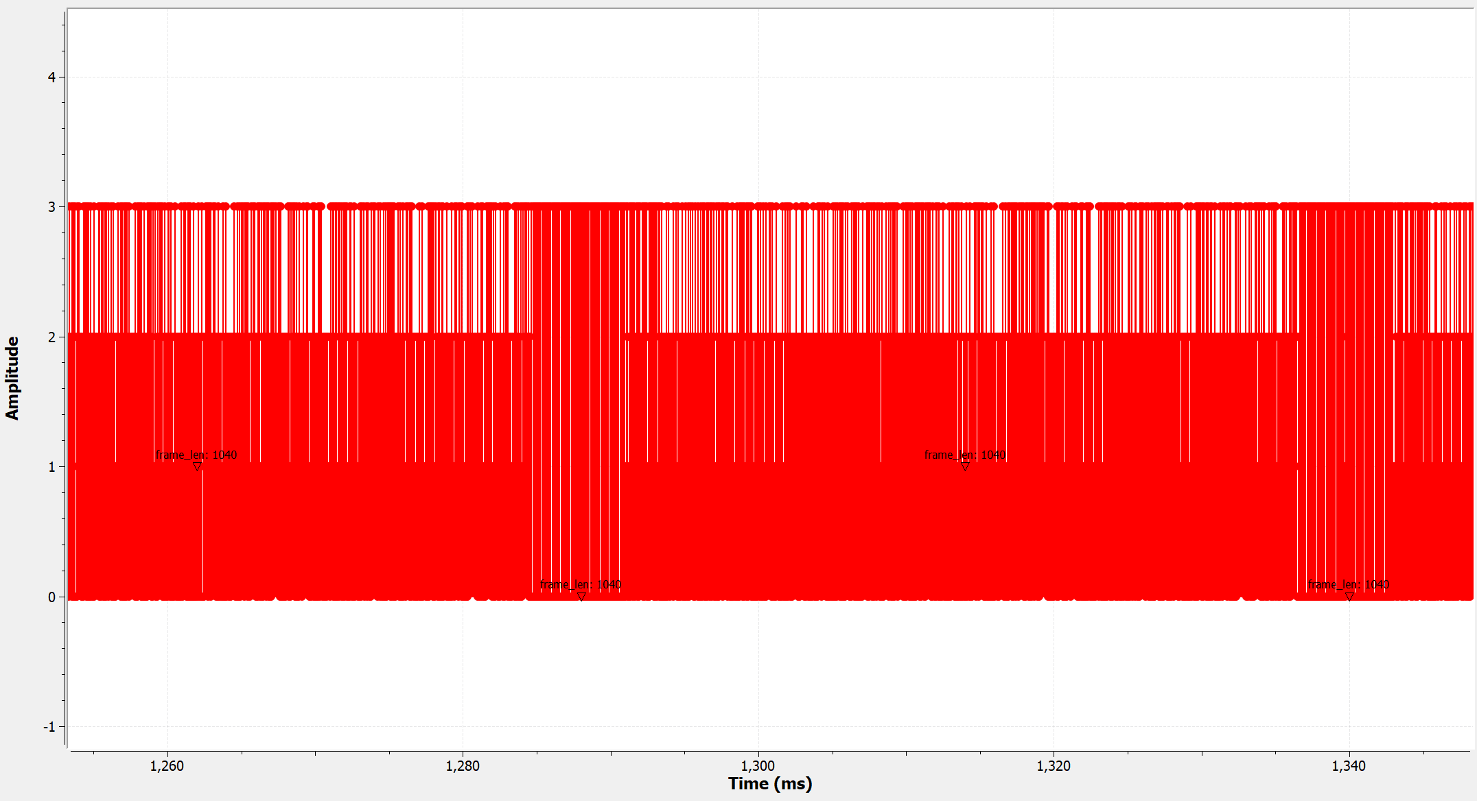
Looking at the output of this block, we see that the values are now restricted to [0,3], corresponding to {00, 01, 10, 11} in binary. Furthermore, each packet that was originally 260 samples long has now become 1080 samples long, since each of the original sample has now been split into 4 consecutive samples.
Another important step to perform before we map our data (and CRC) stream to a QPSK constellation is to generate headers for each packet. The header acts as sort of a metadata for the data packet, telling us information such as the length of the packet and the packet number, which helps the receiver reconstruct the data stream later. The header also includes a (smaller) CRC code for itself to guard against errors. For each data packet, we generate a corresponding header using the “Protocol Formatter” block. The exact format of the header depends on the header format object used.In this example, we are using the built-in header_format_ofdm class.
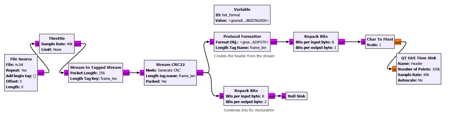
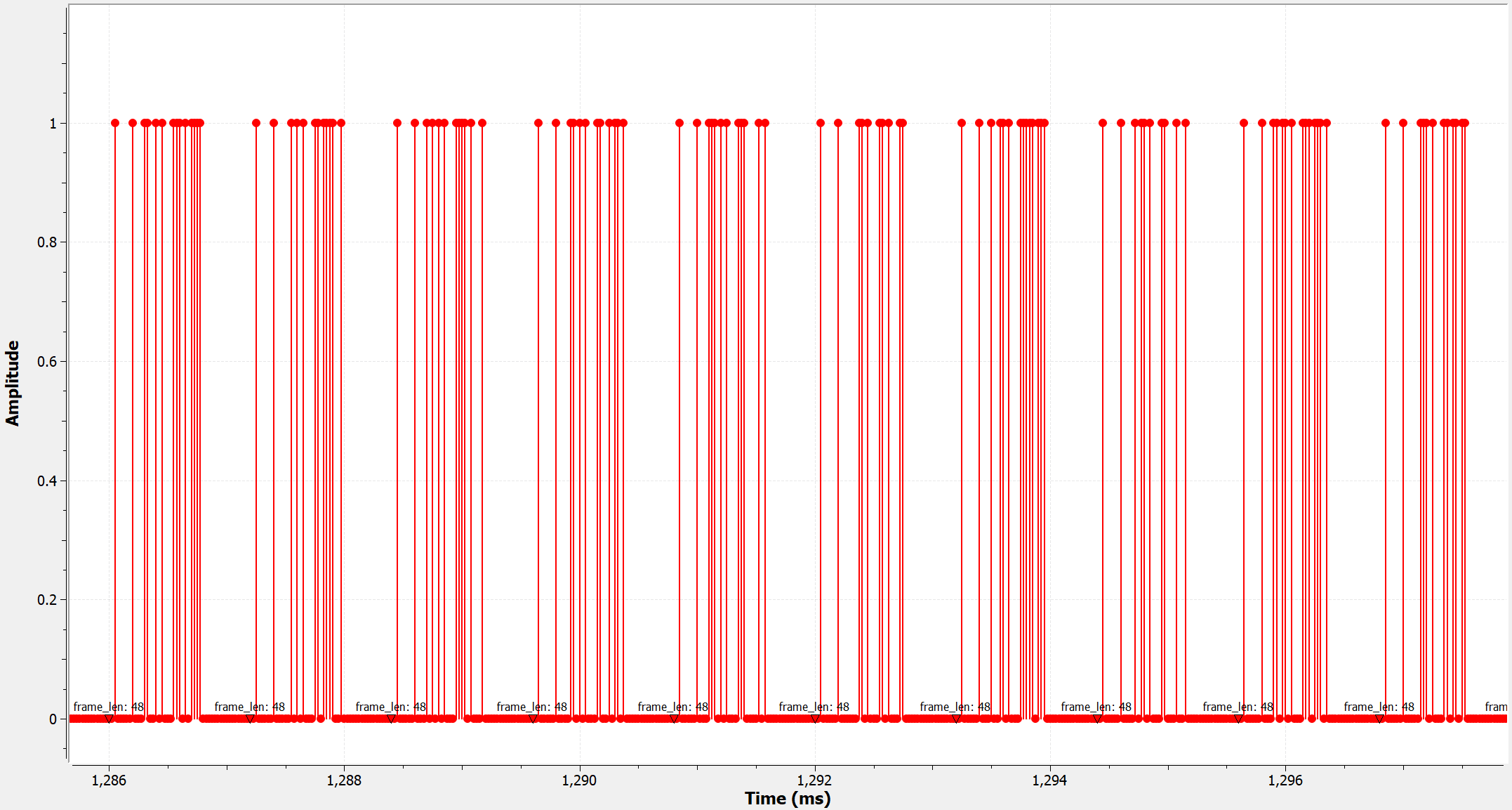
The output of the Protocol Formatter is 8-bit. We repack it into 1-bit binary representation, so that the header may be transmitted using BPSK modulation. Looking at the output of the Protocol Formatter, we see a stream of 48-bit long headers.
Looking at the repacked headers, we see a stream of 48-bit long packets. Notice that even though our data packets are repeated indefinitely by the file source block, the headers are never repeated. This is because the headers contain information unique to each packet, such as the packet number.
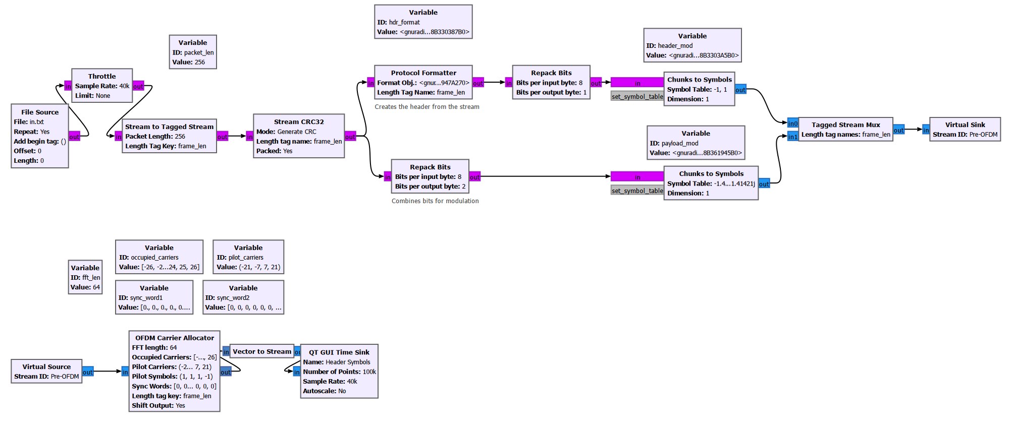
We now have a data stream that consists of values between [0, 3], and a header stream with values between [0, 1]. In order to transmit them using QAM, we must map them to the correct QPSK and BPSK constellation respectively. This is done using the “Chunks to Symbols” block. As can be seen below, each of these blocks takes the symbol table for the desired modulation format, and maps the input samples to a constellation point (a complex number).
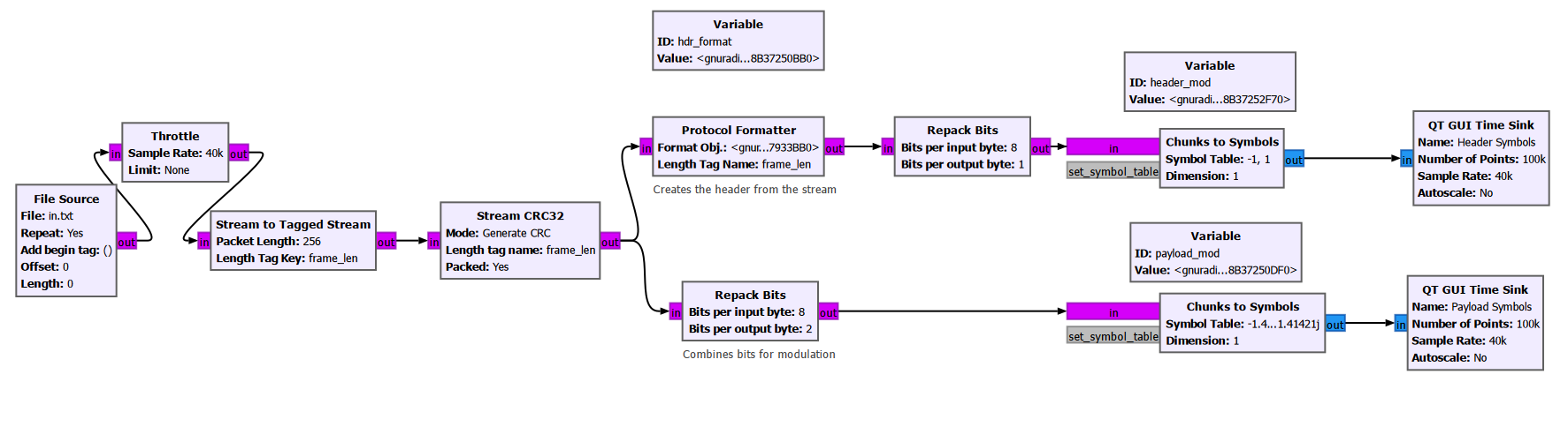
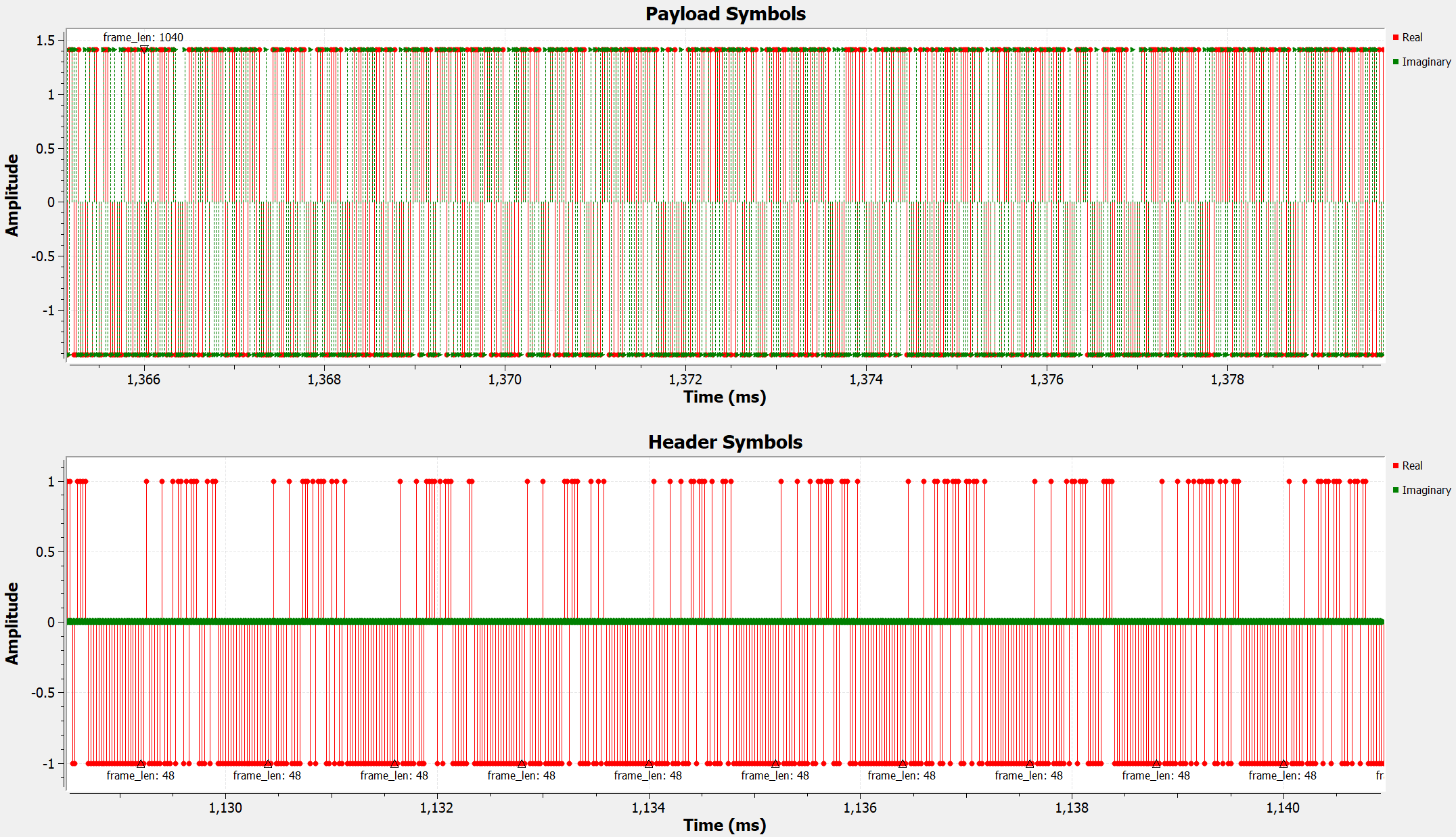
Looking at the output of the symbol maps, we see that the 0s and 1s of the header stream has been converted to -1s and 1s. The 2-bit chunks of the data stream (00, 01, 10, 11) have been mapped to the QPSK constellation points following the table here.
Next we stitch the payload stream and the header stream together using the “Tagged Stream Mux” block. This block takes two inputs sequentially, switching back and forth between the two, and outputs a single combined stream. This way, we end up with a single stream in which each payload packet is preceded by its corresponding header.
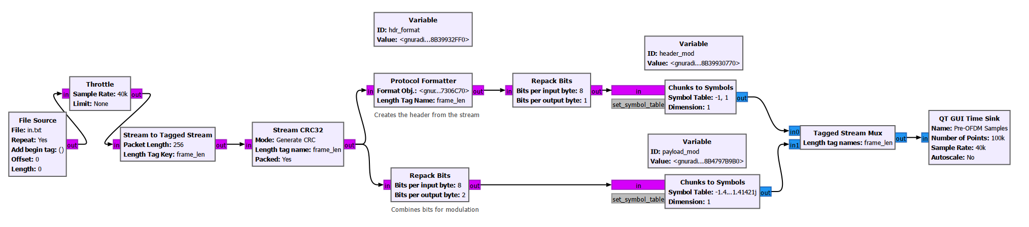
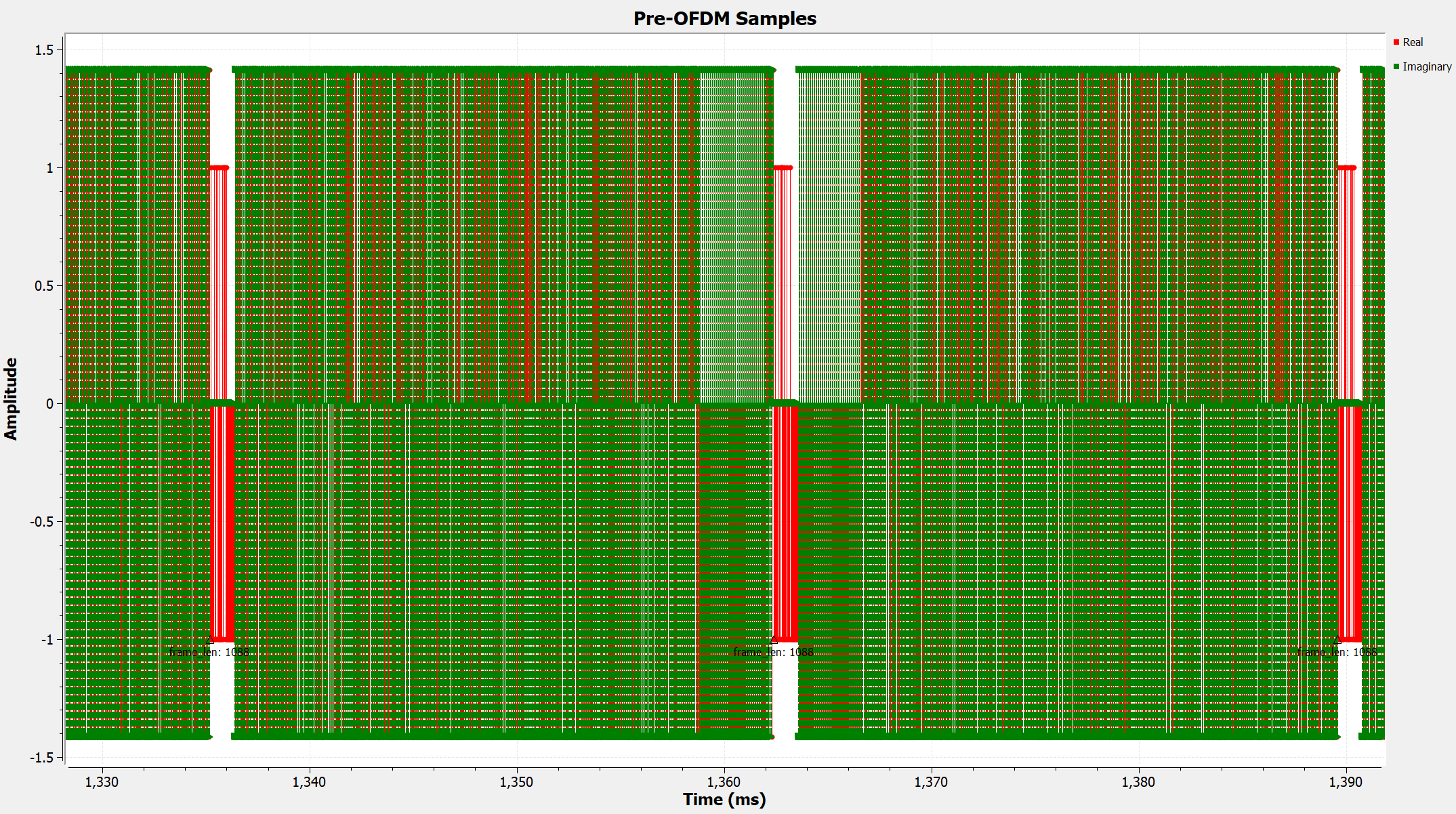
After muxing, we see that each packet is now 1088 samples long. This is because each header packet is 48 samples long, and the payload packet is 1040 samples long. Furthermore, we see that each packet begins with a short sequence of BPSK symbols (header), which is followed by a longer sequence of QPSK symbols (payload).
We are now ready to construct the OFDM radio frames. We will do so using the “OFDM Preallocator Block”.
We have chosen an “FFT length” of 64. This means each OFDM symbol will be consist of up to 64 individual tones (also known as sub-carriers) in the frequency domain, with indices from -32 to 31. Each sub-carrier will have a complex amplitude, corresponding to the complex amplitude of the QAM symbols of our transmit stream. In practice, not all 64 sub-carriers will be used to carry data. We specify which ones will be used through the “Occupied Sub-carriers” argument. In this example, we will use a total of 48 carrier to convey data. Their indices are as follows:
\[[-26:1:-22], [-20:1:-8], [-6,:1:-1], [1:1:6], [8:1:20], [22:1:26]\]In addition to the occupied sub-carriers, we will also allocate 4 pilot sub-carriers. These are tones with complex amplitudes known to both the transmitter and the receiver. They will be used to perform channel estimation and equalization at the receiver. In this example, we chose sub-carriers $[-21, -7, 7, 21]$ as pilot sub-carriers.
The unallocated sub-carriers will have zero amplitude. These are the sub-carriers with the lowest and the highest frequencies, with indices smaller than -26 and greater than 26 respectively. These are also known as the guard sub-carriers. Furthermore, the DC sub-carrier (with index 0) is also left unused.
With the above in mind, the process to construct one OFDM symbol is as follows: we take 48 QAM symbols from our transmit stream, insert them at the occupied sub-carrier. Then, we insert the 4 pilot symbols at the pilot carrier spots. This leaves 64-48-4=12 unused sub-carriers. The 64 samples will be converted from frequency domain to time domain later using an IFFT block.
Since each of our (header+payload) packet consists of 1088 QAM symbols, and 48 QAM symbols can fit inside one OFDM symbol according to our chosen frequency allocation scheme, we will need a total of 23 OFDM symbols (rounded up from 22.6) to transmit the entire packet.
Besides these 23 symbols, we also need to add two “Sync Words” to our radio frame. The sync words are sequences known to both the transmitter and the receiver. They are used to help the receiver perform carrier frequency offset (CFO), sampling frequency offset (SFO) estimation and timing synchronization. So in total, our radio frame will have 25 symbols.
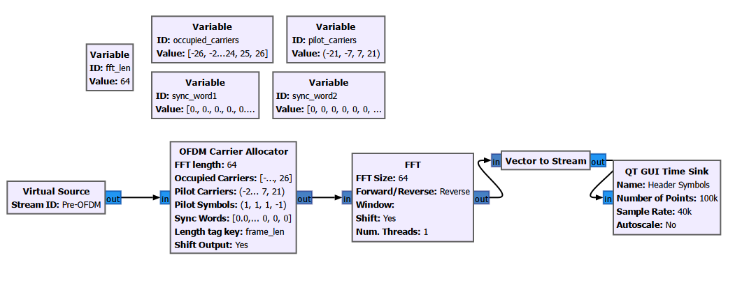
Prior to performing the IFFT, each of the symbol is described by a 64-sample complex vector which describes its FFT (i.e. its frequency spectrum). We can visualize these vectors using the “Vector to Stream” block. This block takes a sequence of vectors and the input, and outputs the samples of the vectors sequentially as a stream.
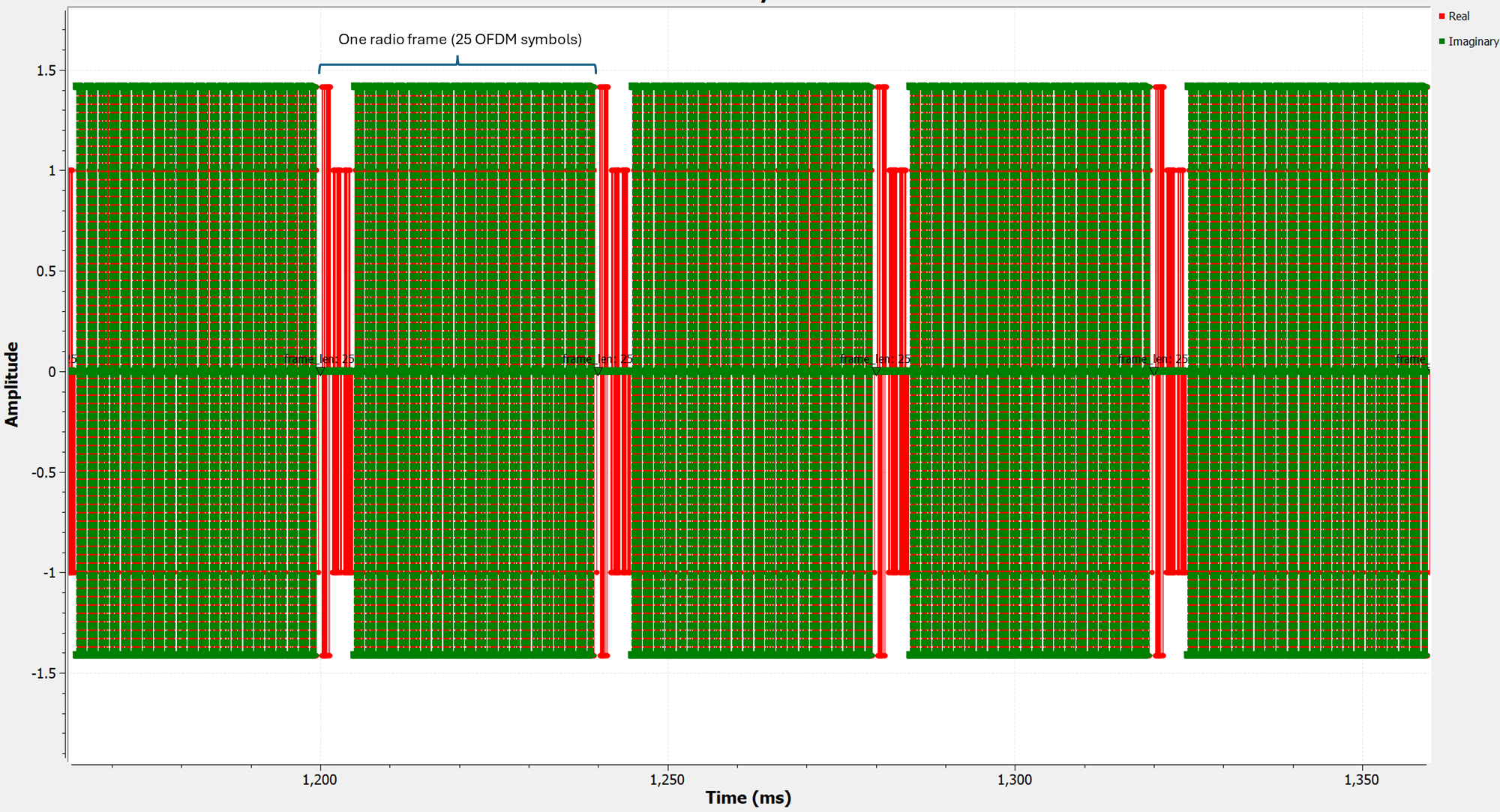
Let’s zoom into a single radio frame and examine its content.
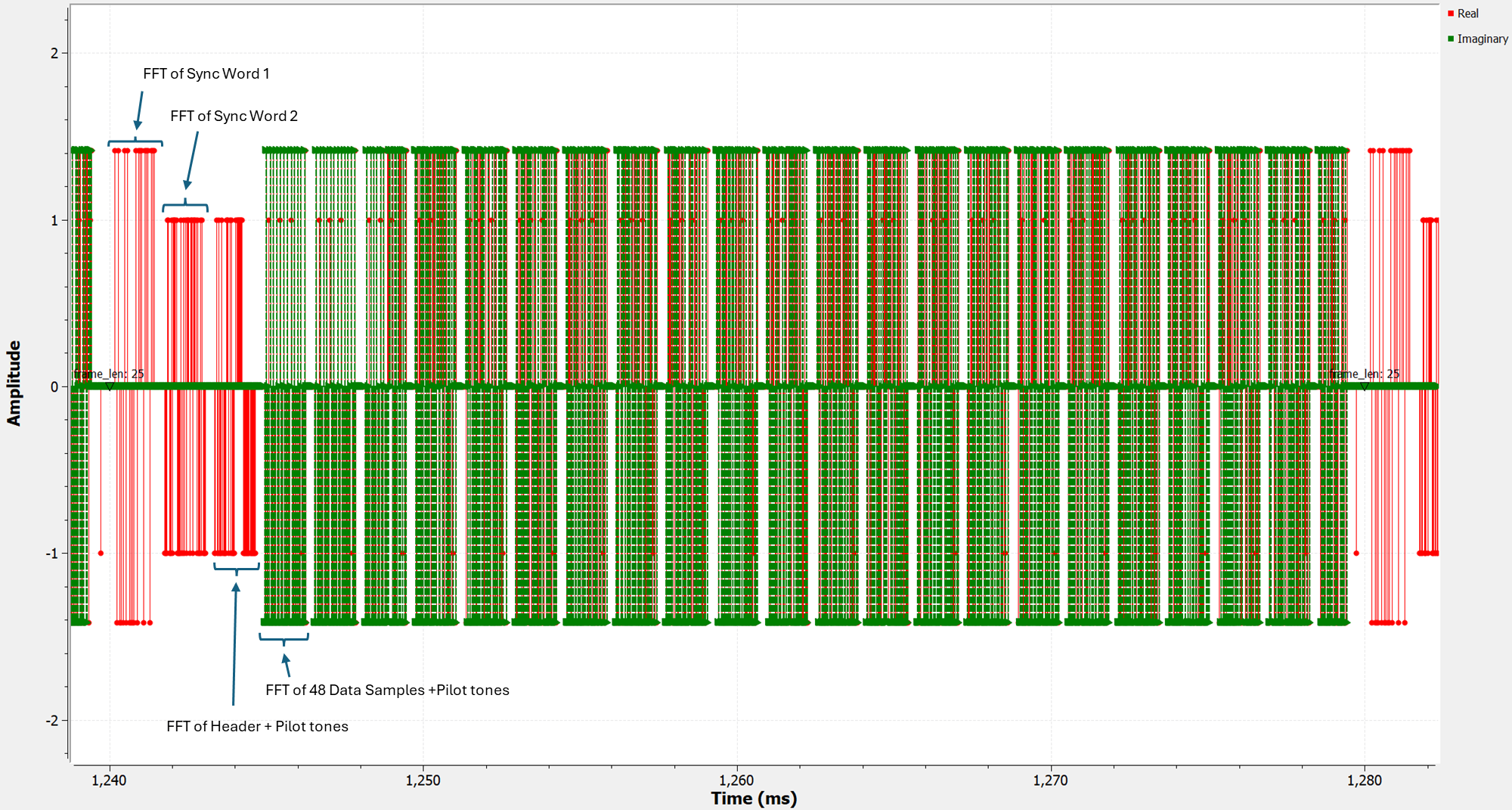
Remember that this is not the actual transmitted time-domain signal. We have simply stitched together 25 frequency domain symbols (i.e. their FFT) and displayed them sequentially.
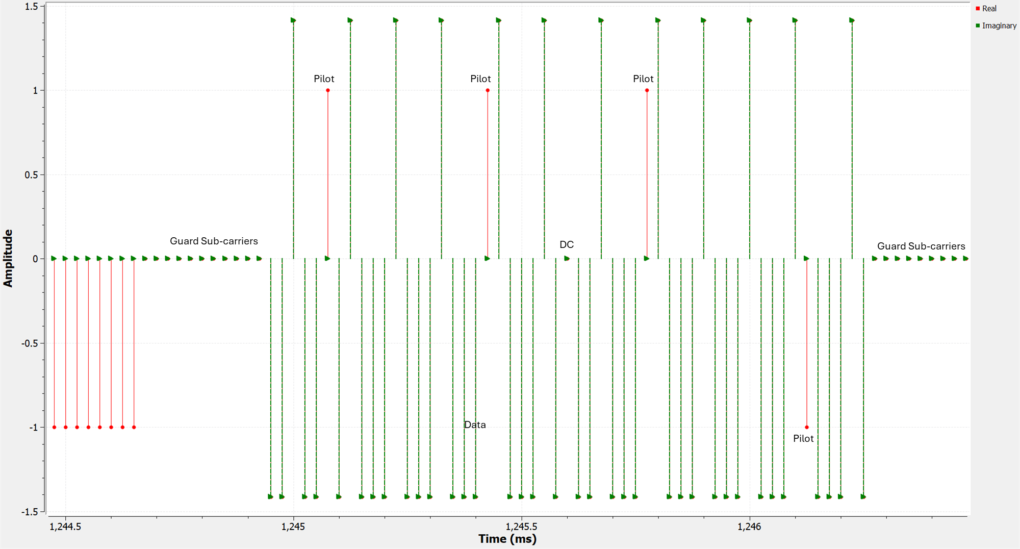
Zooming in further to one of the OFDM data symbols, we can clearly see the guard sub-carriers (zero-amplitude), the data sub-carriers (QPSK modulation), and the pilot sub-carriers (constant values 1 or -1).
In order to transmit this radio frame, we need to convert the symbols from frequency domain to time domain. This is done using the “IFFT” block.
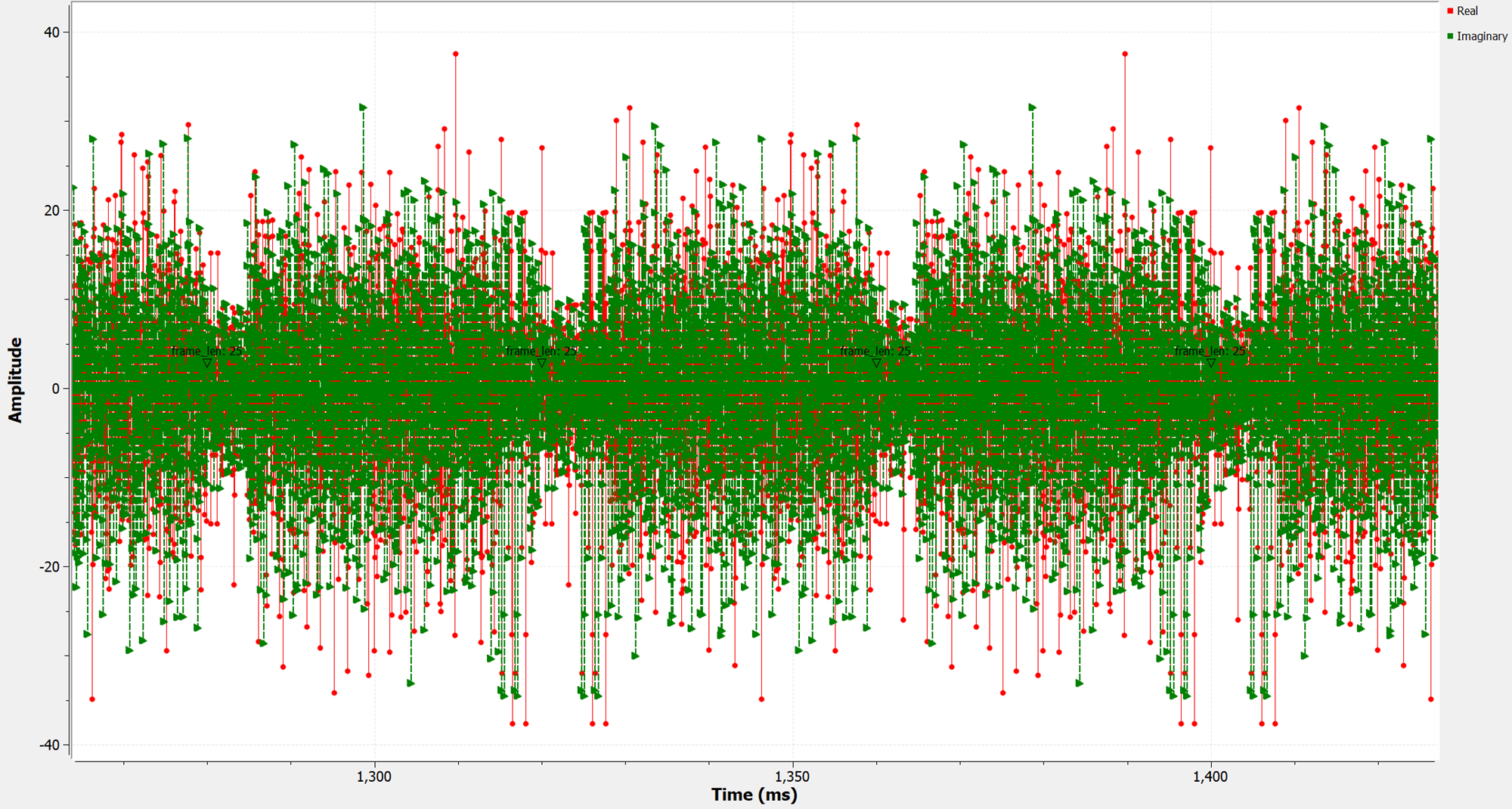
After IFFT, the sequence of complex vectors is as follows
Note that we still do not have a true time-domain waveform. What we have now is a bunch of time-domain OFDM symbols that are stitched together and displayed sequentially using the Vector to Stream block. Before producing the true time-domain waveform, we need to add cyclic prefix to each of the OFDM symbols. That essentially means we take the last N samples of each symbol (16 samples in this example), and prepend it to the beginning of the symbol. I won’t go into the details of the cyclic prefix, but it is an extremely important part of OFDM which acts as a guard interval between adjacent symbols to prevent inter-symbol interference due to multi-path, and enables efficient equalization techniques (one-tap equalization) at the receiver.
We can add cyclic prefix to each time-domain symbol using the “OFDM Cyclic Prefixer” block.
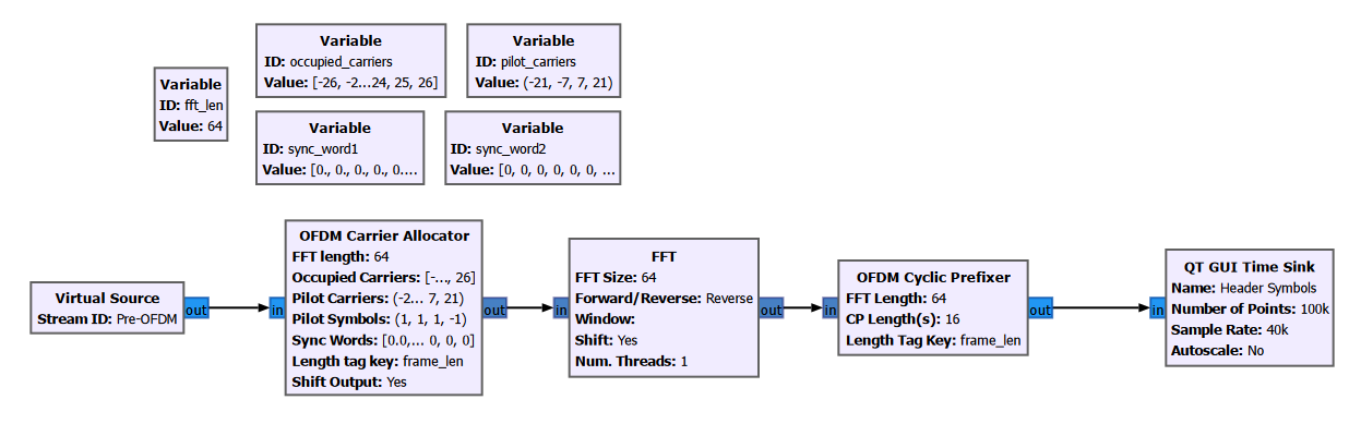
This block also takes the prepended symbols and generates a true time-domain waveform:
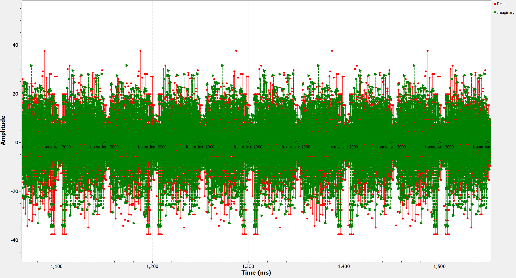
Notice that each radio frame now consists of 2000 samples. This is because each symbol is 64 samples long, with 16 samples of cyclic prefix. We have 25 total symbols including two sync words. As a reminder, our original file is 512 byte long, and each frame holds 256 bytes of data; so our file is will be transmitted over the course of 2 radio frames.
The final processing step in the baseband before upconversion to radiofrequency (RF) is to upsample and interpolate the OFDM waveform. The low-sample-rate waveform generates many imaged copies of the basedband spectrum in the frequency domain which are difficult to filter out post digital-to-analog conversion (DAC) efficiently using analog filters. Instead, if we upsample the waveform and interpolate it, the images are pushed further apart in frequency, allowing us to filter them out using much simpler filters with less stringent roll-off requirements.
Let us take a look at the upsampled time-domain OFDM waveform, as well as its frequency spectrum.
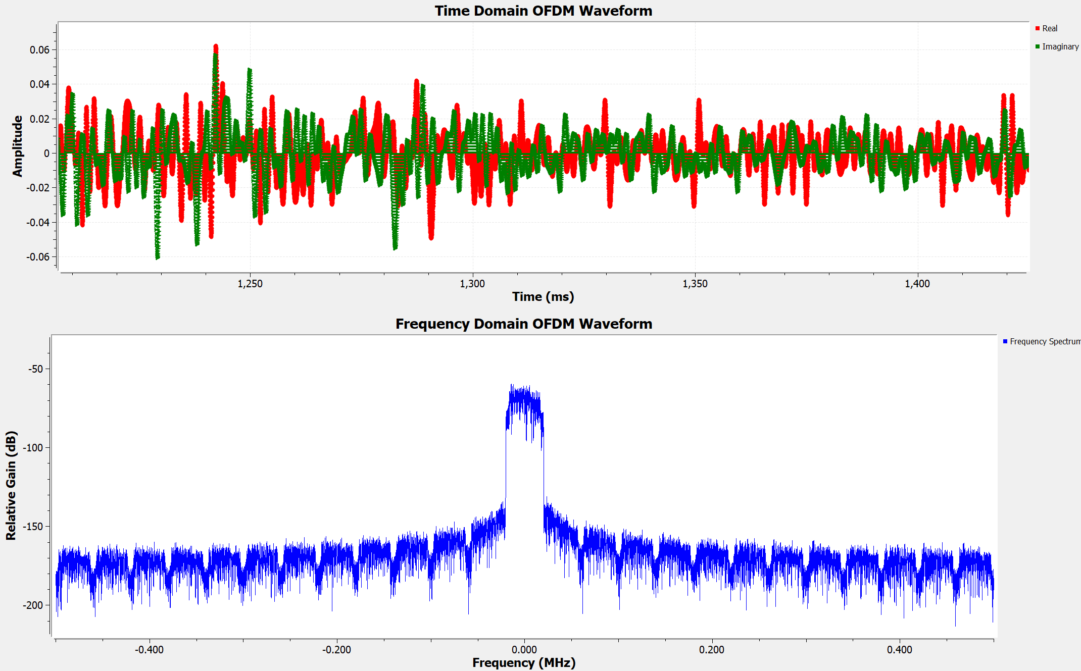
In the above time-domain OFDM waveform, we can also see that the peak amplitude is very large compared to its average amplitude. Hence the waveform has a high peak-to-average ratio (PAPR). This is a known problem for OFDM systems, which limits their efficiency (in particular the efficiency of the amplifiers).
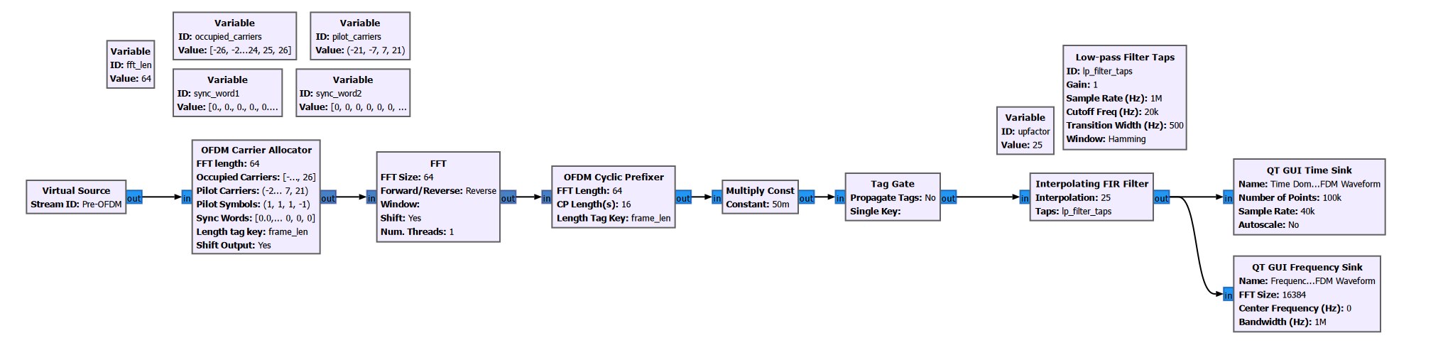
Finally, before transmitting the signal over-the-air, we need to upconvert it to a higher frequency, so that it can be radiated efficiently using an antenna. For now, since we are just simulating the system without any actual hardware, we will do the up-conversion digitally, by multiplying the real and the imaginary part of the signal with a sine and a consine wave at the carrier frequency. This is exactly how an IQ mixer works. So the completely transmitter chain looks like this:
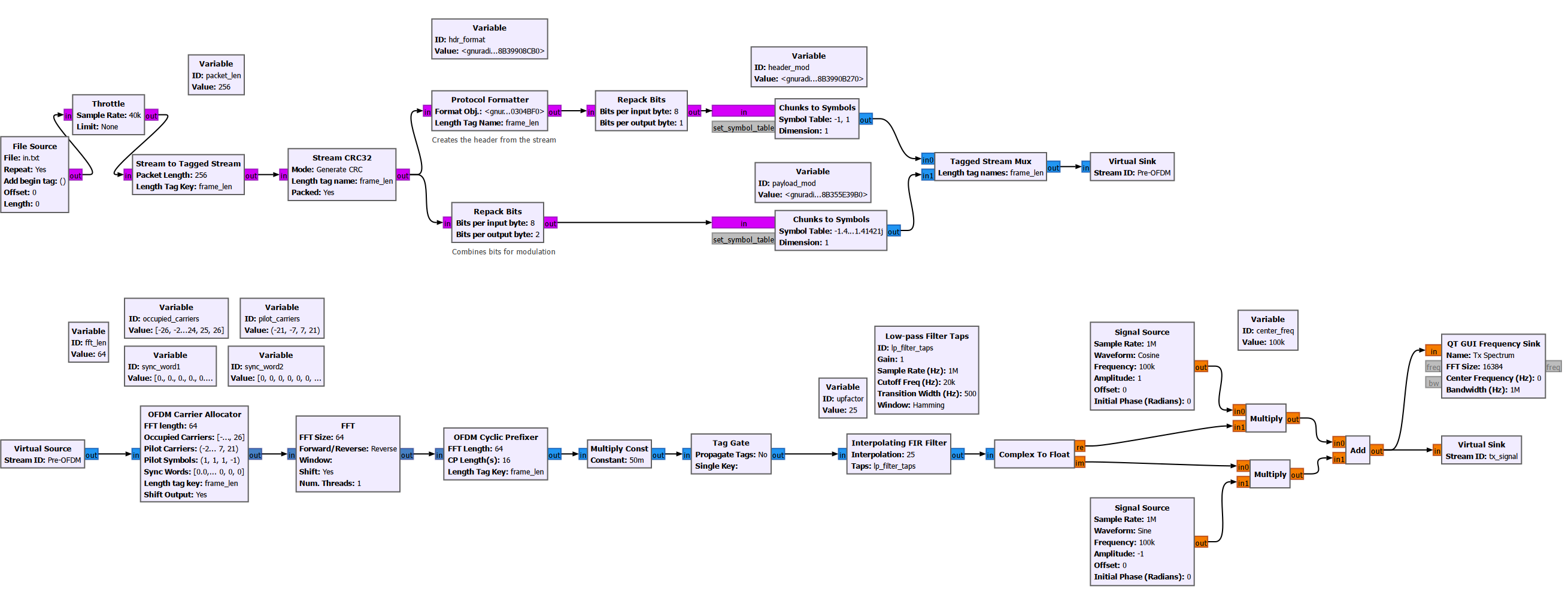
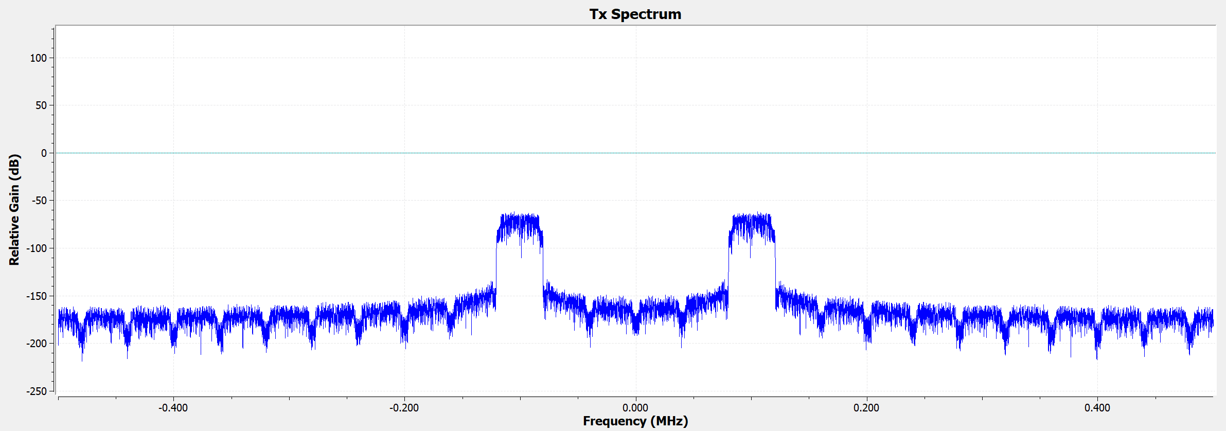
At the output of our digital IQ mixer, we can see that the energy of the signal is now centered at the carrier frequency (chosen to be 100kHz for illustration; we will use a much higher frequency when actually transmitting the signal over-the-air).
1.2 Receiver
At the receiver, our first task is to downconvert the signal from RF to baseband. Again, since we are only simulating the system now, we will perform this operating digitally.
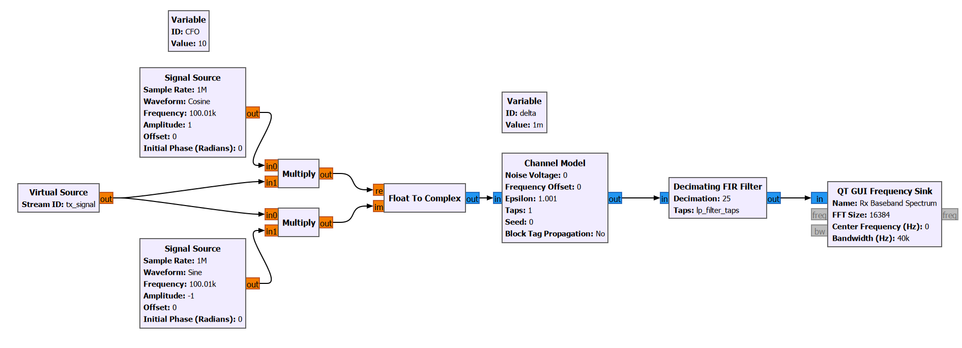
Notice that the carrier frequency of the receiver does not match that of the transmitter exactly, because I have manually added a carrier frequency offset (CFO). CFO is present in any real communication system due to mismatch between the transmitter and the receiver local oscillator frequencies, the doppler effect, etc.
After downconversion using the digital mixer, I have added a “Channel Model” block, which is used to simulate the effect of timing offset between the transmitter and the receiver.
Notice that prior to down-sampling the signal for further digital processing, we apply a low pass filter (LPF). The LPF that we applied is exactly the same as the interpolating LPF used at the transmitter. This is called matched filtering. It helps ensure we get the maximum possible signal-to-noise ratio (SNR) at the receiver when transmitting over a noisy channel.
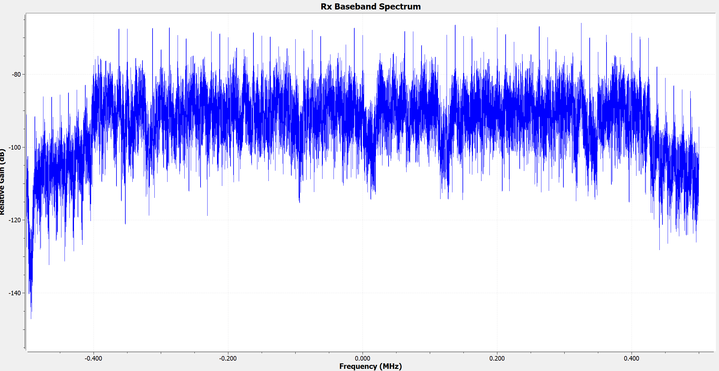
The downsampled received basedband signal has the following frequency spectrum:
In order to properly demodulate the received signal, we must estimate the CFO perform a coarse correction. Otherwise the demodulated constellation points will keep rotating on the IQ plane, preventing us from properly translating the points back into bits. I will not go over the exact working principle of the CFO estimator here. I will just show that we can do so using the “Schmidl & Cox OFDM Synchronization” block.
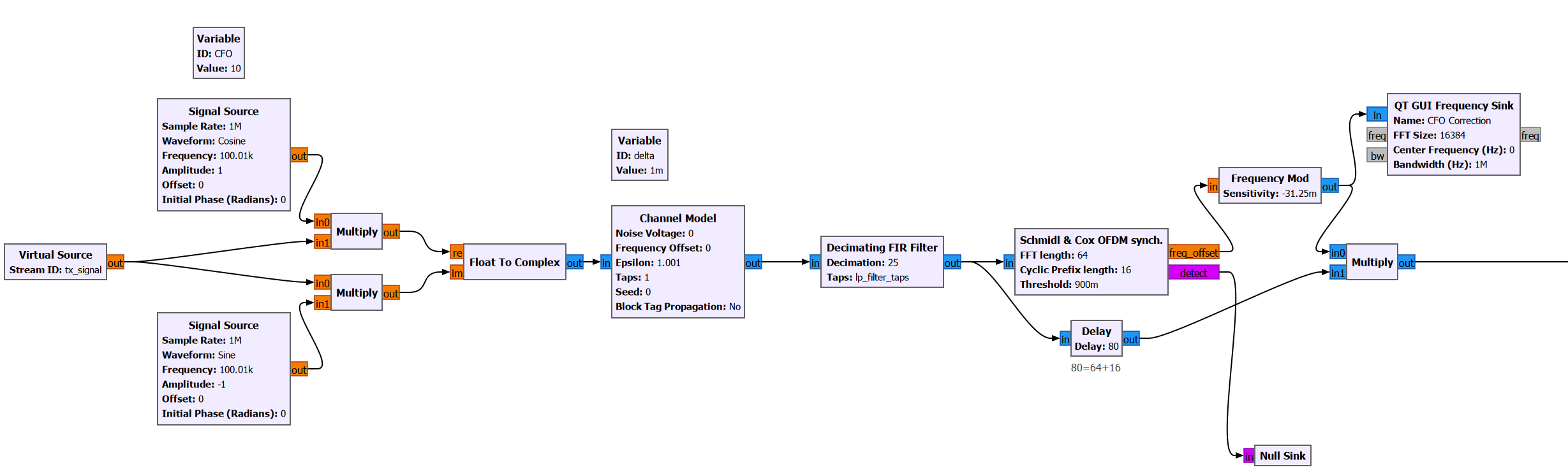
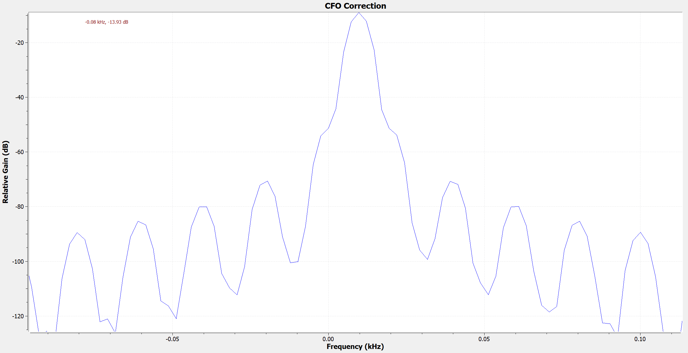
Essentially, this block estimates and outputs the carrier frequency offset. Using the “Frequency Mod” block, we generate a complex sinusoid whose frequency is equal to the negative of the offset frequency. Then, when we multiply the original signal (with the CFO) with this sinusoid, the frequency offset is cancelled out.
This is made clear when we plot the output spectrum of the Frequency Mod block; It is a complex sinusoid (i.e. its spectrum is not symmetric) with frequency 10Hz. Since our receiver has an LO frequency of 100.010kHz, the downconverted baseband signal will be centered around -10Hz. After multiplying with this sinusoid, the baseband signal will be centered around 0Hz.
This step only achieves coarse CFO correction. We will perform fine CFO correction at a later stage using the synchronization words that were added to the radio frames.
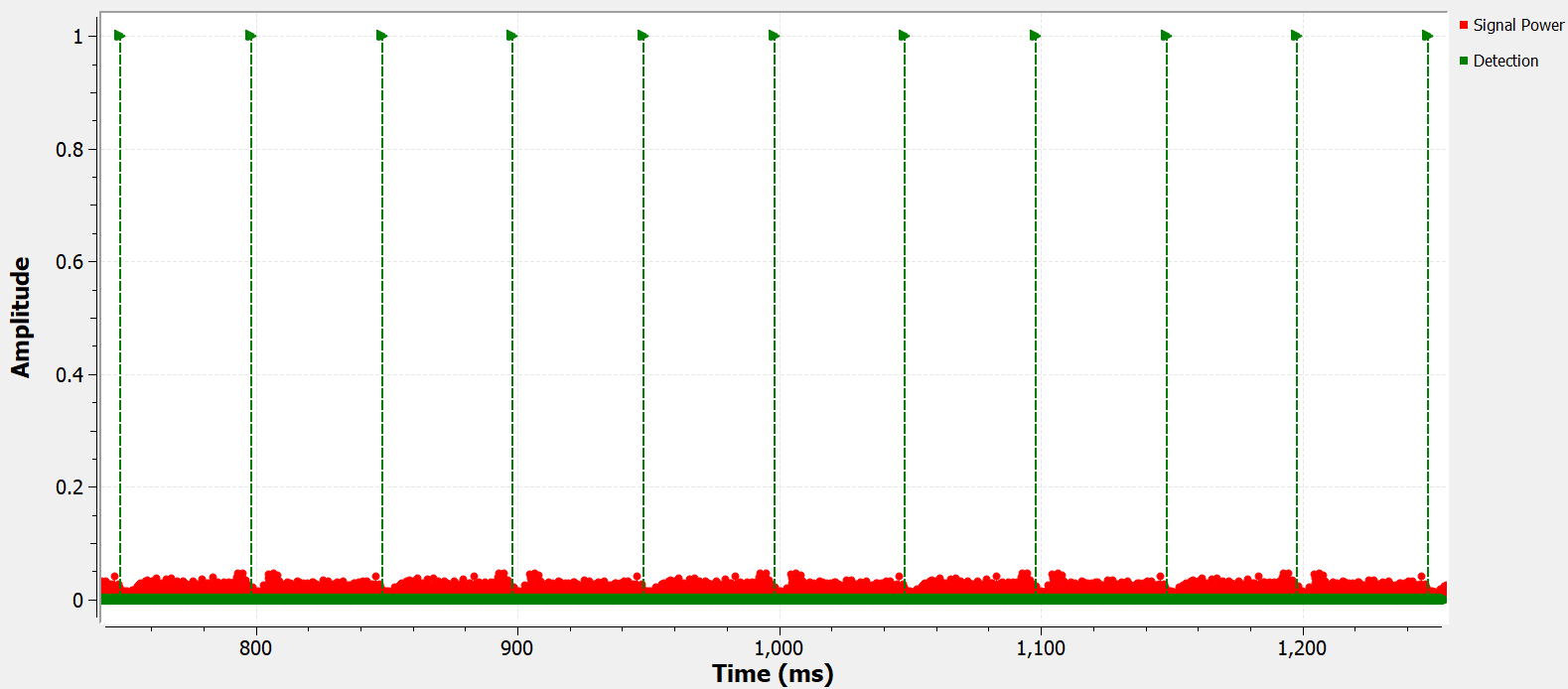
Another important output of the OFDM Sychronization block is the “Detect” flag, which is raised to 1 every time a new radio frame is detected.
If we plot the time domain signal and the detect flag together, we can see that the flag aligns with the radio frames. (remember our signal is essentially 2 radio frames that are repeated indefinitely).
We tell the block that there are 3 header symbols. These correspond to the two sync words and the one preamble symbol which we added using the Protocol Formatter in the TX chain.
2 Experiment with Hardware
I will first attempt to transmit and receive some OFDM packets using a bladeRF 2.0 micro xA4 which has a loopback mode. This will be easier than trying to transmit and receive over-the-air using two separate HackRFs, since we do not need to worry about CFO and SFO.